Variable Transformations in R: Understanding Distributions and Data Cleaning

Introduction

Political science data rarely comes in perfect, analysis-ready form. Before running any statistical analyses, you’ll often need to transform your variables to make them more suitable for modeling or to better understand their underlying patterns. This tutorial will walk you through essential variable transformation techniques, focusing on why these transformations matter for political science research.

By the end of this tutorial, you’ll understand:

How to identify and interpret different types of distributions
When and why to apply logarithmic transformations
Essential techniques for recoding categorical variables
Best practices for handling missing data and outliers

Setting Up: Loading Libraries and Data

library(tidyverse)

── Attaching core tidyverse packages ──────────────────────── tidyverse 2.0.0 ──
✔ dplyr     1.1.4     ✔ readr     2.1.5
✔ forcats   1.0.0     ✔ stringr   1.5.1
✔ ggplot2   3.5.2     ✔ tibble    3.3.0
✔ lubridate 1.9.4     ✔ tidyr     1.3.1
✔ purrr     1.1.0     
── Conflicts ────────────────────────────────────────── tidyverse_conflicts() ──
✖ dplyr::filter() masks stats::filter()
✖ dplyr::lag()    masks stats::lag()
ℹ Use the conflicted package (<http://conflicted.r-lib.org/>) to force all conflicts to become errors

library(scales)


Attaching package: 'scales'

The following object is masked from 'package:purrr':

    discard

The following object is masked from 'package:readr':

    col_factor

set.seed(1234)  # For reproducible examples

For this tutorial, we’ll work with both simulated data and a real-world example using country-level political and economic indicators.

# Create sample data that mimics real political science variables
countries <- data.frame(
  country = paste("Country", 1:100),
  gdp_per_capita = rlnorm(100, meanlog = 8, sdlog = 1.5),  # Log-normal distribution
  population = rlnorm(100, meanlog = 15, sdlog = 2),       # Highly skewed
  democracy_score = rbeta(100, 2, 2) * 10,                # Bounded 0-10
  election_turnout = rnorm(100, 65, 15),                   # Normal-ish
  regime_type = sample(c("Democracy", "Hybrid", "Autocracy"), 100,
                      prob = c(0.4, 0.3, 0.3), replace = TRUE)
)

head(countries)

    country gdp_per_capita population democracy_score election_turnout
1 Country 1      487.55416  7489758.2        6.349214         58.29560
2 Country 2     4519.44222  1264975.2        6.907414         76.44765
3 Country 3    15163.73142  3730254.4        5.522234         87.07578
4 Country 4       88.36301  1196659.4        6.917598         71.65497
5 Country 5     5674.21231   626561.9        5.874055         58.67417
6 Country 6     6368.27453  4565225.9        7.069599         64.39998
  regime_type
1   Democracy
2      Hybrid
3   Autocracy
4   Autocracy
5   Democracy
6   Democracy

Part 1: Understanding Distributions

What Do Distributions Tell Us?

The distribution of a variable shows us how values are spread across the range of possible outcomes. In political science, understanding distributions helps us:

Choose appropriate statistical methods
Identify unusual cases or outliers
Make valid comparisons across groups
Communicate findings effectively

Visualizing Distributions

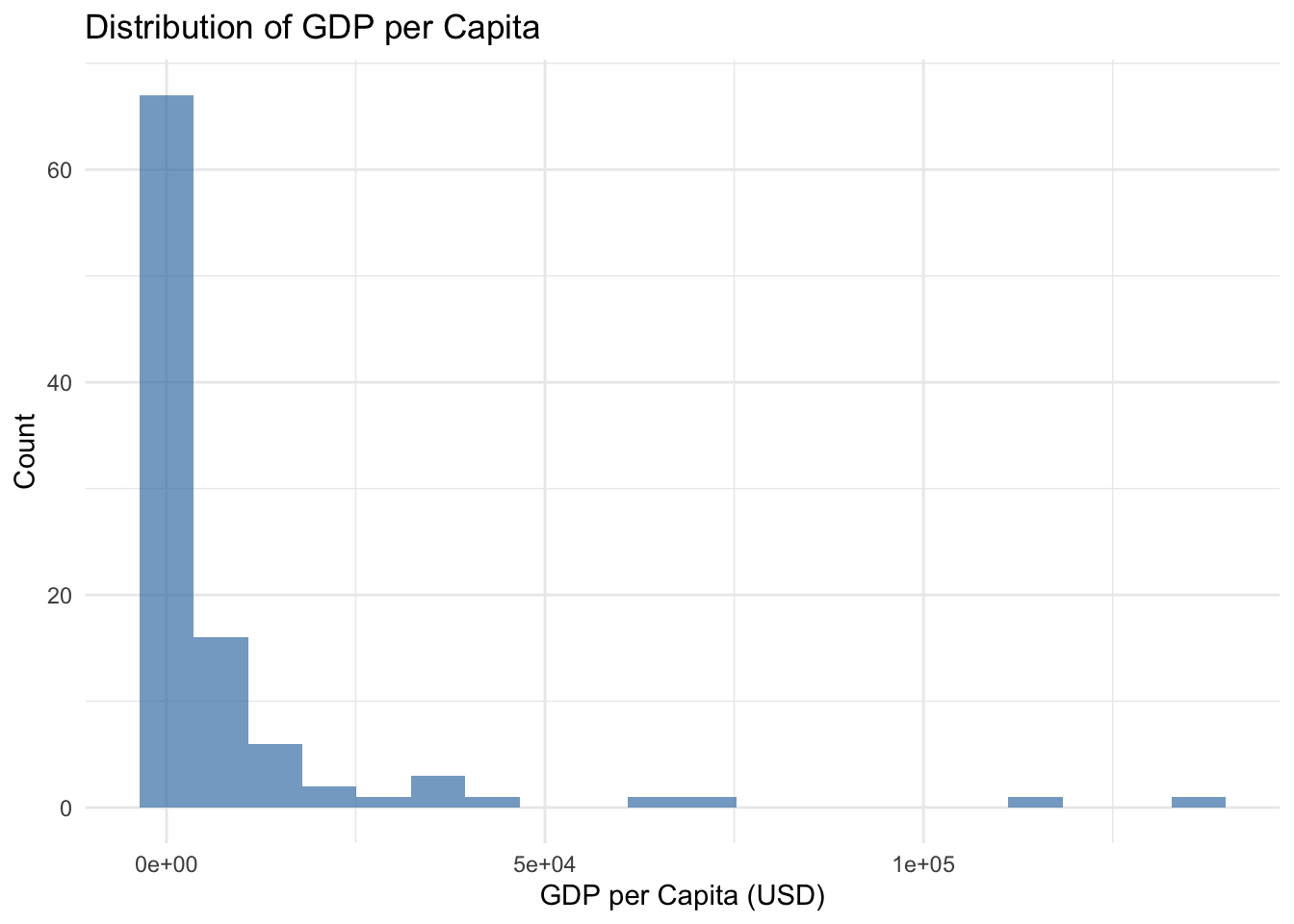
Let’s examine the distribution of GDP per capita in our sample:

# Basic histogram
countries %>%
  ggplot(aes(x = gdp_per_capita)) +
  geom_histogram(bins = 20, fill = "steelblue", alpha = 0.7) +
  labs(title = "Distribution of GDP per Capita",
       x = "GDP per Capita (USD)",
       y = "Count") +
  theme_minimal()

What do you notice? The distribution is heavily right-skewed—most countries cluster at lower GDP levels, with a few very wealthy countries creating a long right tail.

Types of Distributions in Political Science

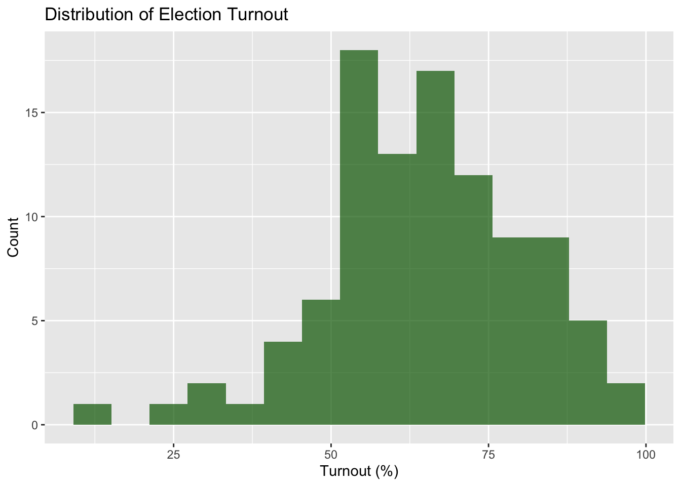
Normal Distribution: Symmetric, bell-shaped curve. Many statistical tests assume normality.

# Election turnout - closer to normal
countries %>%
  ggplot(aes(x = election_turnout)) +
  geom_histogram(bins = 15, fill = "darkgreen", alpha = 0.7) +
  labs(title = "Distribution of Election Turnout",
       x = "Turnout (%)",
       y = "Count")

Skewed Distributions: Common with economic variables, population sizes, conflict casualties.

# Population - highly right-skewed
countries %>%
  ggplot(aes(x = population)) +
  geom_histogram(bins = 20, fill = "coral", alpha = 0.7) +
  labs(title = "Distribution of Population",
       x = "Population",
       y = "Count") +
  scale_x_continuous(labels = label_scientific())

Part 2: The Power of Logarithmic Transformations

Why Log Transformations Matter

Logarithmic transformations are crucial in political science because they:

Reduce skewness in right-skewed distributions
Stabilize variance across different scales
Make relationships linear that are otherwise exponential
Allow meaningful interpretation of percentage changes

When to Use Log Transformations

Use log transformations when:

Variables span several orders of magnitude (GDP, population, military spending)
You observe exponential relationships
You want to interpret effects as percentage changes
The variable has a long right tail

Applying Log Transformations

# Add log-transformed variables
countries <- countries %>%
  mutate(
    log_gdp = log(gdp_per_capita),
    log_population = log(population)
  )

Comparing Original vs. Log-Transformed

# Create side-by-side comparison
p1 <- countries %>%
  ggplot(aes(x = gdp_per_capita)) +
  geom_histogram(bins = 20, fill = "steelblue", alpha = 0.7) +
  labs(title = "Original GDP per Capita", x = "GDP per Capita") +
  theme_minimal()

p2 <- countries %>%
  ggplot(aes(x = log_gdp)) +
  geom_histogram(bins = 20, fill = "steelblue", alpha = 0.7) +
  labs(title = "Log GDP per Capita", x = "Log(GDP per Capita)") +
  theme_minimal()

# Display plots side by side (you might need gridExtra package)
# grid.arrange(p1, p2, ncol = 2)

Key Insight: The log transformation converts the right-skewed distribution into something much closer to normal!

Interpreting Log-Transformed Variables

When you use log-transformed variables in regression:

A 1-unit change in log(X) represents a 100% increase in X
A 0.1-unit change in log(X) represents approximately a 10% increase in X
This makes economic interpretations much more intuitive

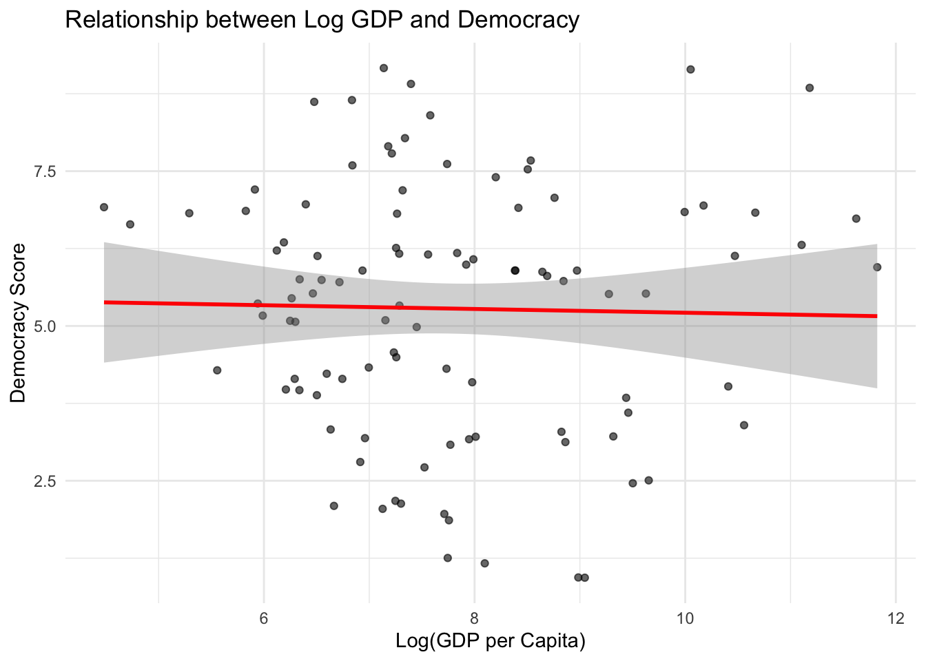
# Example: How does log GDP relate to democracy scores?
countries %>%
  ggplot(aes(x = log_gdp, y = democracy_score)) +
  geom_point(alpha = 0.6) +
  geom_smooth(method = "lm", color = "red") +
  labs(title = "Relationship between Log GDP and Democracy",
       x = "Log(GDP per Capita)",
       y = "Democracy Score") +
  theme_minimal()

`geom_smooth()` using formula = 'y ~ x'

Part 3: Recoding Variables

Why Recode Variables?

Recoding involves changing how variables are categorized or valued. Common reasons:

Simplifying analysis: Converting continuous variables to categories
Fixing data problems: Standardizing inconsistent coding
Creating meaningful groups: Collapsing small categories
Handling missing data: Deciding how to treat different types of missingness

Creating Categorical Variables from Continuous Ones

# Create GDP categories
countries <- countries %>%
  mutate(
    gdp_category = case_when(
      gdp_per_capita < 5000 ~ "Low Income",
      gdp_per_capita < 20000 ~ "Middle Income",
      gdp_per_capita >= 20000 ~ "High Income"
    ),
    # Alternative using quantiles
    gdp_tertile = case_when(
      gdp_per_capita <= quantile(gdp_per_capita, 0.33) ~ "Bottom Third",
      gdp_per_capita <= quantile(gdp_per_capita, 0.67) ~ "Middle Third",
      TRUE ~ "Top Third"
    )
  )

# Check the distribution
table(countries$gdp_category)


  High Income    Low Income Middle Income 
           11            72            17

Recoding Categorical Variables

# Sometimes you need to collapse categories
countries <- countries %>%
  mutate(
    simple_regime = case_when(
      regime_type == "Democracy" ~ "Democratic",
      regime_type %in% c("Hybrid", "Autocracy") ~ "Non-Democratic"
    )
  )

table(countries$simple_regime)


    Democratic Non-Democratic 
            43             57

Creating Dummy Variables

For regression analysis, you often need to convert categorical variables into numeric dummy variables:

# Create dummy variables for regime types
countries <- countries %>%
  mutate(
    is_democracy = ifelse(regime_type == "Democracy", 1, 0),
    is_hybrid = ifelse(regime_type == "Hybrid", 1, 0),
    is_autocracy = ifelse(regime_type == "Autocracy", 1, 0)
  )

# Check correlations (should be negative - if one is 1, others are 0)
cor(countries[c("is_democracy", "is_hybrid", "is_autocracy")])

             is_democracy  is_hybrid is_autocracy
is_democracy    1.0000000 -0.5416386   -0.5550941
is_hybrid      -0.5416386  1.0000000   -0.3985498
is_autocracy   -0.5550941 -0.3985498    1.0000000

Part 4: Handling Missing Data and Outliers

Identifying Missing Data Patterns

# Introduce some missing data for demonstration
countries_with_missing <- countries %>%
  mutate(
    # Randomly assign some missing values
    democracy_score = ifelse(runif(n()) < 0.1, NA, democracy_score),
    election_turnout = ifelse(runif(n()) < 0.05, NA, election_turnout)
  )

# Check missing data patterns
summary(countries_with_missing)

   country          gdp_per_capita        population        democracy_score 
 Length:100         Min.   :    88.36   Min.   :1.081e+04   Min.   :0.9347  
 Class :character   1st Qu.:   778.29   1st Qu.:1.071e+06   1st Qu.:3.9636  
 Mode  :character   Median :  1674.76   Median :3.491e+06   Median :5.7426  
                    Mean   :  8739.23   Mean   :3.223e+07   Mean   :5.3331  
                    3rd Qu.:  6046.71   3rd Qu.:1.147e+07   3rd Qu.:6.8295  
                    Max.   :136419.04   Max.   :1.439e+09   Max.   :9.1644  
                                                            NA's   :11      
 election_turnout regime_type           log_gdp       log_population  
 Min.   :14.06    Length:100         Min.   : 4.481   Min.   : 9.288  
 1st Qu.:55.15    Class :character   1st Qu.: 6.657   1st Qu.:13.881  
 Median :64.25    Mode  :character   Median : 7.423   Median :15.066  
 Mean   :63.95                       Mean   : 7.765   Mean   :15.082  
 3rd Qu.:73.24                       3rd Qu.: 8.707   3rd Qu.:16.255  
 Max.   :98.78                       Max.   :11.823   Max.   :21.088  
 NA's   :8                                                            
 gdp_category       gdp_tertile        simple_regime       is_democracy 
 Length:100         Length:100         Length:100         Min.   :0.00  
 Class :character   Class :character   Class :character   1st Qu.:0.00  
 Mode  :character   Mode  :character   Mode  :character   Median :0.00  
                                                          Mean   :0.43  
                                                          3rd Qu.:1.00  
                                                          Max.   :1.00  
                                                                        
   is_hybrid     is_autocracy 
 Min.   :0.00   Min.   :0.00  
 1st Qu.:0.00   1st Qu.:0.00  
 Median :0.00   Median :0.00  
 Mean   :0.28   Mean   :0.29  
 3rd Qu.:1.00   3rd Qu.:1.00  
 Max.   :1.00   Max.   :1.00

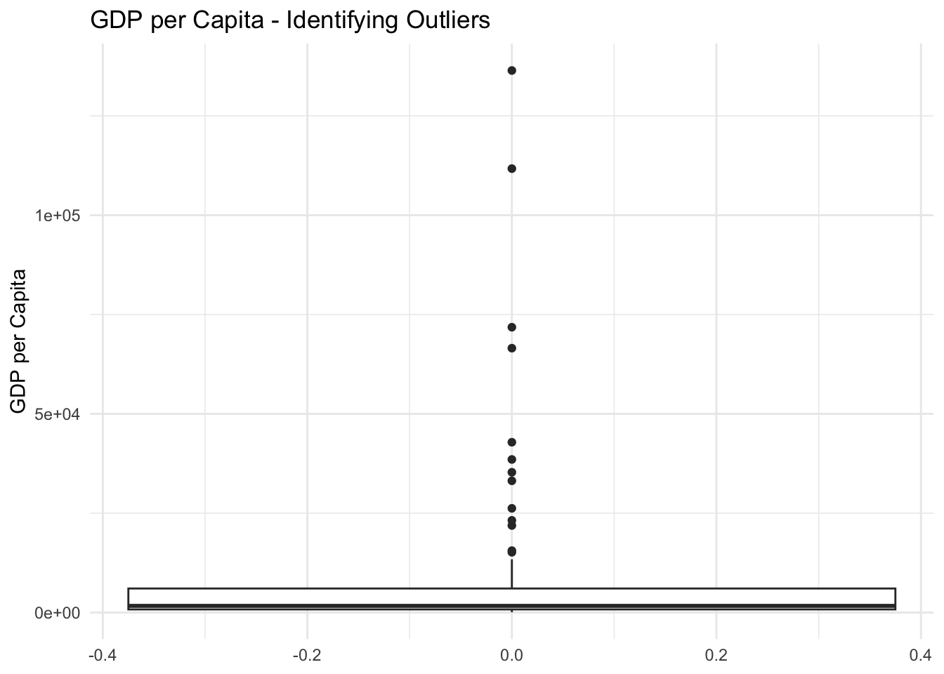
Identifying Outliers

# Box plot to identify outliers
countries %>%
  ggplot(aes(y = gdp_per_capita)) +
  geom_boxplot() +
  labs(title = "GDP per Capita - Identifying Outliers",
       y = "GDP per Capita") +
  theme_minimal()

# Statistical approach: values beyond 1.5 * IQR
outlier_threshold <- quantile(countries$gdp_per_capita, 0.75) +
                     1.5 * IQR(countries$gdp_per_capita)

countries %>%
  filter(gdp_per_capita > outlier_threshold) %>%
  select(country, gdp_per_capita)

       country gdp_per_capita
1    Country 3       15163.73
2   Country 20      111720.20
3   Country 31       15575.37
4   Country 41       26219.13
5   Country 57       35303.11
6   Country 59       33152.20
7   Country 62      136419.04
8   Country 66       42857.10
9   Country 68       23196.13
10  Country 69       21902.31
11  Country 75       66529.87
12  Country 93       38520.51
13 Country 100       71802.58

Handling Outliers

# Option 1: Remove outliers (use cautiously!)
countries_no_outliers <- countries %>%
  filter(gdp_per_capita <= outlier_threshold)

# Option 2: Winsorize (cap at certain percentiles)
countries_winsorized <- countries %>%
  mutate(
    gdp_winsorized = case_when(
      gdp_per_capita > quantile(gdp_per_capita, 0.95) ~ quantile(gdp_per_capita, 0.95),
      gdp_per_capita < quantile(gdp_per_capita, 0.05) ~ quantile(gdp_per_capita, 0.05),
      TRUE ~ gdp_per_capita
    )
  )

Part 5: Best Practices and Common Pitfalls

Documentation is Key

# Always document your transformations
countries_final <- countries %>%
  mutate(
    # Log transformation for skewed economic variables
    log_gdp_pc = log(gdp_per_capita),  # Natural log of GDP per capita
    log_pop = log(population),         # Natural log of population

    # Standardized democracy score (0-1 scale)
    democracy_01 = democracy_score / 10,

    # Binary regime classification
    democratic = ifelse(regime_type == "Democracy", 1, 0)
  ) %>%
  # Keep original variables for comparison
  select(country, gdp_per_capita, log_gdp_pc, democracy_score, democracy_01,
         regime_type, democratic, everything())

Common Mistakes to Avoid

Taking logs of zero or negative values - Add a small constant if necessary
Over-transforming - Not every skewed variable needs transformation
Losing track of original scales - Keep both versions when possible
Mechanical outlier removal - Investigate outliers before removing them

Checking Your Work

# Always examine your transformations
summary(countries_final[c("gdp_per_capita", "log_gdp_pc", "democracy_score", "democracy_01")])

 gdp_per_capita        log_gdp_pc     democracy_score   democracy_01    
 Min.   :    88.36   Min.   : 4.481   Min.   :0.9347   Min.   :0.09347  
 1st Qu.:   778.29   1st Qu.: 6.657   1st Qu.:3.8713   1st Qu.:0.38713  
 Median :  1674.76   Median : 7.423   Median :5.7161   Median :0.57161  
 Mean   :  8739.23   Mean   : 7.765   Mean   :5.2812   Mean   :0.52812  
 3rd Qu.:  6046.71   3rd Qu.: 8.707   3rd Qu.:6.8229   3rd Qu.:0.68229  
 Max.   :136419.04   Max.   :11.823   Max.   :9.1644   Max.   :0.91644

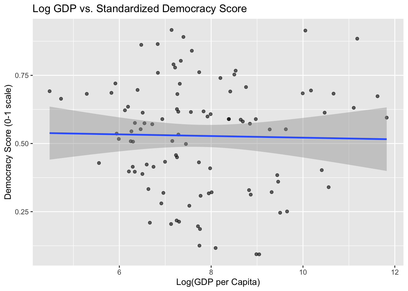
# Visualize relationships
countries_final %>%
  ggplot(aes(x = log_gdp_pc, y = democracy_01)) +
  geom_point(alpha = 0.6) +
  geom_smooth(method = "lm") +
  labs(title = "Log GDP vs. Standardized Democracy Score",
       x = "Log(GDP per Capita)",
       y = "Democracy Score (0-1 scale)")

`geom_smooth()` using formula = 'y ~ x'

Conclusion

Variable transformations are fundamental tools in political science research. Key takeaways:

Understand your data first - Always visualize distributions before transforming
Log transformations are powerful for right-skewed economic/demographic variables
Thoughtful recoding can simplify analysis and improve interpretation
Document everything - Future you will thank present you
Keep originals - Preserve untransformed variables for robustness checks