Tutorial 3: Grouping, Filtering, Mutating, Selecting, and Plotting

The everyday verbs of data manipulation in dplyr

Almost everything you will do with data in this course is some combination of four verbs: group rows together, filter rows out, mutate new columns into existence, and summarize what is left. This tutorial walks through each one, then plots the result.

The data

In class we load an extract from the American National Election Studies. So that the code on this page runs on your machine without the course data file, we will build a small simulated stand-in with the same variable names. Everything below works identically on the real data — just swap in the load() line from the course files.

library(tidyverse)

set.seed(2075)

n <- 400
nes <- tibble(
  vote12 = sample(
    c("Barack Obama", "Mitt Romney", "Did not vote"),
    size = n, replace = TRUE, prob = c(0.42, 0.38, 0.20)
  ),
  age = round(rnorm(n, mean = 49, sd = 16)),
  educ_years = round(rnorm(n, mean = 14, sd = 2.5))
) |>
  mutate(
    ftobama = case_when(
      vote12 == "Barack Obama" ~ rnorm(n, 78, 14),
      vote12 == "Mitt Romney"  ~ rnorm(n, 27, 16),
      vote12 == "Did not vote" ~ rnorm(n, 50, 20)
    ),
    # feeling thermometers are bounded at 0 and 100
    ftobama = pmin(pmax(round(ftobama), 0), 100)
  )

summary() is the first thing to run on any new dataset. It tells you the type of each column, the range of the numeric ones, and — importantly — how many values are missing.

nes |>
  summary()

    vote12               age          educ_years       ftobama      
 Length:400         Min.   :10.00   Min.   : 6.00   Min.   :  0.00  
 Class :character   1st Qu.:35.75   1st Qu.:12.75   1st Qu.: 30.00  
 Mode  :character   Median :48.00   Median :14.00   Median : 53.00  
                    Mean   :48.06   Mean   :14.25   Mean   : 51.81  
                    3rd Qu.:58.00   3rd Qu.:16.00   3rd Qu.: 73.00  
                    Max.   :93.00   Max.   :22.00   Max.   :100.00  

Summarize

summarize() collapses many rows into one. Ask it for the mean feeling thermometer score toward Obama across the whole sample:

nes |>
  summarize(mean_ftobama = mean(ftobama))

# A tibble: 1 × 1
  mean_ftobama
         <dbl>
1         51.8

Group, then summarize

On its own that number hides everything interesting. group_by() tells summarize() to compute the statistic separately within each category — this is how you get comparisons rather than aggregates.

nes |>
  group_by(vote12) |>
  summarize(mean_ftobama = mean(ftobama))

# A tibble: 3 × 2
  vote12       mean_ftobama
  <chr>               <dbl>
1 Barack Obama         76.2
2 Did not vote         48.0
3 Mitt Romney          27.9

Filter

filter() keeps only the rows that satisfy a condition. Note the double equals sign: == asks a question, while a single = assigns a value.

nes |>
  filter(vote12 == "Barack Obama") |>
  summarize(mean_ftobama = mean(ftobama))

# A tibble: 1 × 1
  mean_ftobama
         <dbl>
1         76.2

Mutate

mutate() adds a column. It can be a constant, though that is rarely useful:

nes |>
  mutate(new_var = "this is a new variable") |>
  glimpse()

Rows: 400
Columns: 5
$ vote12     <chr> "Barack Obama", "Did not vote", "Did not vote", "Barack Oba…
$ age        <dbl> 26, 54, 60, 30, 71, 55, 27, 43, 18, 54, 72, 37, 62, 57, 59,…
$ educ_years <dbl> 9, 15, 13, 15, 15, 15, 17, 10, 13, 15, 19, 16, 13, 13, 11, …
$ ftobama    <dbl> 100, 49, 47, 94, 92, 46, 79, 75, 42, 26, 60, 91, 31, 6, 43,…
$ new_var    <chr> "this is a new variable", "this is a new variable", "this i…

More often you want a column that is a function of existing columns. case_when() is the workhorse for recoding a continuous variable into categories — read each line as “condition ~ value”.

nes |>
  mutate(ftobama_cat = case_when(
    ftobama >= 50 ~ "Generally Positive",
    ftobama < 50  ~ "Generally Negative"
  )) |>
  glimpse()

Rows: 400
Columns: 5
$ vote12      <chr> "Barack Obama", "Did not vote", "Did not vote", "Barack Ob…
$ age         <dbl> 26, 54, 60, 30, 71, 55, 27, 43, 18, 54, 72, 37, 62, 57, 59…
$ educ_years  <dbl> 9, 15, 13, 15, 15, 15, 17, 10, 13, 15, 19, 16, 13, 13, 11,…
$ ftobama     <dbl> 100, 49, 47, 94, 92, 46, 79, 75, 42, 26, 60, 91, 31, 6, 43…
$ ftobama_cat <chr> "Generally Positive", "Generally Negative", "Generally Neg…

Nothing you have done so far has changed nes itself. Piping into glimpse() prints a result and throws it away. To keep the new column, assign the result back:

nes <- nes |>
  mutate(ftobama_cat = case_when(
    ftobama >= 50 ~ "Generally Positive",
    ftobama < 50  ~ "Generally Negative"
  ))

Plot

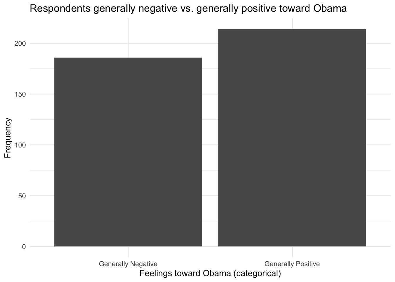
Now that the categorical variable exists, ggplot2 can count it. geom_bar() does the tabulation for you, so you only supply the x variable.

g <- nes |>
  ggplot(aes(x = ftobama_cat)) +
  geom_bar()

g +
  theme_minimal() +
  labs(
    x = "Feelings toward Obama (categorical)",
    y = "Frequency",
    title = "Respondents generally negative vs. generally positive toward Obama"
  )

Recap

• summarize() collapses rows into statistics; group_by() makes it do so within categories.
• filter() selects rows, select() selects columns, mutate() creates columns.
• Nothing is saved unless you assign it with <-.
• ggplot2 expects tidy data — the recoding you do with mutate() is what makes the plot possible.

Next: variable transformations, where recoding gets more consequential for your inferences. The full series is on the tutorials page.